Gromov-Wasserstein Correspondences

Overview

GWProt treats proteins as point clouds in 3-dimensional space defined by their alpha-carbons. The Gromov-Wasserstein (GW) distance 1 between two point clouds quantifies how different the two structures are, up to rigid transformations (rotations and translations).

Intuitively, GW compares proteins by structurally aligning their residues in a way that minimizes distortion between their internal distance matrices.

Gromov-Hausdorff Distance

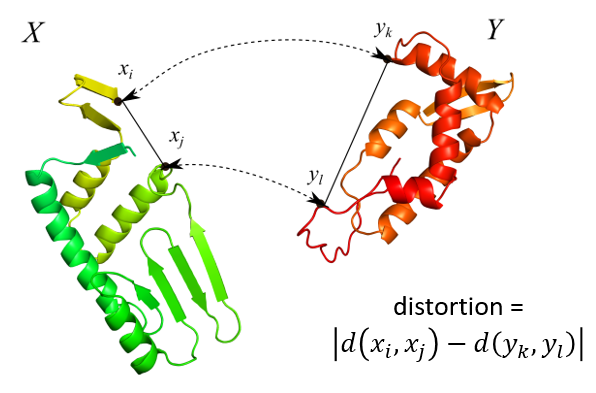
As a starting point, we can form a one-to-one pairing \(f\) between the residues in protein \(X\) and those in protein \(Y\) that minimizes the largest distortion—the difference between a distance within \(X\) and the corresponding distance in \(Y\). This defines the Gromov-Hausdorff distance between \(X\) and \(Y\):

\[GH(X,Y) = \min_{f :X\cong Y} \max_{i,j \in X} | d_X(i,j) - d_Y(f(i),f(j)) |.\]

However, this is not computable in practice, as the number of possibilities for \(f\) grows on the order of \(|X|!\).

Gromov-Wasserstein Distance

To address this, one can turn the problem into a continuous one that can be efficiently approximated. We assign each protein a total mass of 1, distributed evenly among its residues. Aligning two proteins of lengths \(n\) and \(m\) then amounts to transferring the mass of one protein to the other. This assignment is called a correspondence or coupling and is represented as an \(n \times m\) matrix, where each column sums to \(1/m\) and each row sums to \(1/n\). The \((i,j)\)-th entry is the amount of mass transported from the \(i\)-th residue of one protein to the \(j\)-th residue of the other. Finding the best alignment is now equivalent to finding the optimal correspondence.

We define the Gromov-Wasserstein distance based on the sum of all distortions, weighted by the optimal correspondence:

\[GW(X,Y) = \min_T \frac{1}{2} \left( \sum_{i,j,k,l} |d_X(x_i,x_j) - d_Y(y_k,y_l)|^2 T_{i,k}T_{j,l} \right)^{1/2}.\]

This is a mathematical metric in that it satisfies basic axioms analogous to distances. Along with calculating the GW distance, we also obtain the optimal correspondence. The squaring and square root are not mathematically necessary, but are used for efficient computation.

Note

In almost all cases, the calculated approximation is equivalent to the precise GW metric for practical purposes. The key exception is that the calculated approximations do not always satisfy the mathematical properties of the true metric (e.g., the triangle inequality may not hold).

References

1

Mémoli, F. (2011). Gromov–Wasserstein distances and the metric approach to object matching. Foundations of Computational Mathematics, 11(4), 417-487.