Example 2: Detecting topologically non-trivial sequence rearrangements

This example demonstrates how GWProt can identify topological permutations in protein sequences, specifically in viral RNA-dependent RNA polymerases (RdRps).

Riboviruses are a realm of viruses that include many human pathogens. All riboviruses encode an essential RNA-dependent RNA polymerase (RdRp), which is crucial for viral replication, exhibits a high mutation rate, and often shows very low sequence homology. As a result, structural comparison is key for identification and classification.

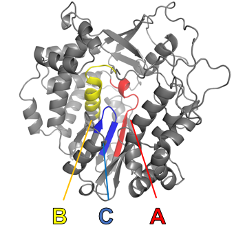
Viral RdRps contain topologically non-trivial permutations across multiple phyla—proteins where the same motifs or domains appear in different orders along the backbone. RdRps have three active site motifs, labeled A, B, and C, which typically appear in the order ABC but can also appear as CAB. We use ‘ABC’ and ‘CAB’ to denote these two types of RdRps.

We first load 10 proteins of each type, with PDB files predicted using AlphaFold.

import os
import numpy as np
import GWProt.GW_protein

dir = 'Example_Data/Permuted Proteins/'
file_list = os.listdir(dir)
ABC_prots = [GWProt.GW_protein.GW_protein.make_protein_from_pdb(os.path.join(dir , file)) for file in file_list if 'abc' in file]
CAB_prots = [GWProt.GW_protein.GW_protein.make_protein_from_pdb(os.path.join(dir , file)) for file in file_list if 'cab' in file]

We then create an LGD_Comparison object and compute all pairwise GW distances using local geometric distortion (LGD).

import GWProt.lgd_comparison

A = GWProt.lgd_comparison.LGD_Comparison(prot_list=ABC_prots + CAB_prots)
A.GW_compute_lgd()

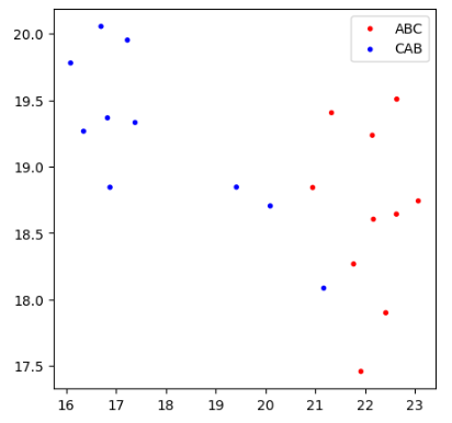
Using UMAP visualization, we observe that proteins can be clustered by permutation type using GW distance, although the separation is weak.

import matplotlib.pyplot as plt
from umap.umap_ import UMAP

reducer = UMAP(metric = 'precomputed')
embedding = reducer.fit_transform(A.get_GW_dmat())
plt.figure(figsize=(5,5))
plt.scatter(embedding[:10,0] ,embedding[:10,1], color = ['red']*10 , s = 8 )
plt.scatter(embedding[10:,0] ,embedding[10:,1], color = ['blue']*10 , s = 8 )
plt.legend(["ABC","CAB" ])

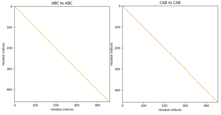
If we examine the correspondence between two ABC proteins or two CAB proteins, it closely resembles the identity matrix, indicating that the GW alignment is nearly sequential.

fig , axes = plt.subplots(nrows = 1, ncols = 2, figsize=(10,10))
fig.tight_layout()

# two ABC proteins
axes[0].imshow(A.transport_dict[A.name_list[0]][A.name_list[1]], cmap = 'hot_r')
axes[0].set_title('ABC to ABC')
axes[0].set_xlabel('residue indices')
axes[0].set_ylabel('residue indices')


#two CAB proteins
axes[1].imshow(A.transport_dict[A.name_list[10]][A.name_list[11]], cmap = 'hot_r')
axes[1].set_title('CAB to CAB')
axes[1].set_xlabel('residue indices')
axes[1].set_ylabel('residue indices')
plt.show()

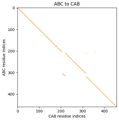
In contrast, the correspondence between an ABC protein and a CAB protein is close to the identity matrix except for a region where the C motifs are aligned.

plt.imshow(A.transport_dict[A.name_list[0]][A.name_list[10]], cmap = 'hot_r', label = 'ABC to CAB')
plt.title('ABC to CAB')
plt.xlabel('CAB residue indices')
plt.ylabel('ABC residue indices')
plt.show()

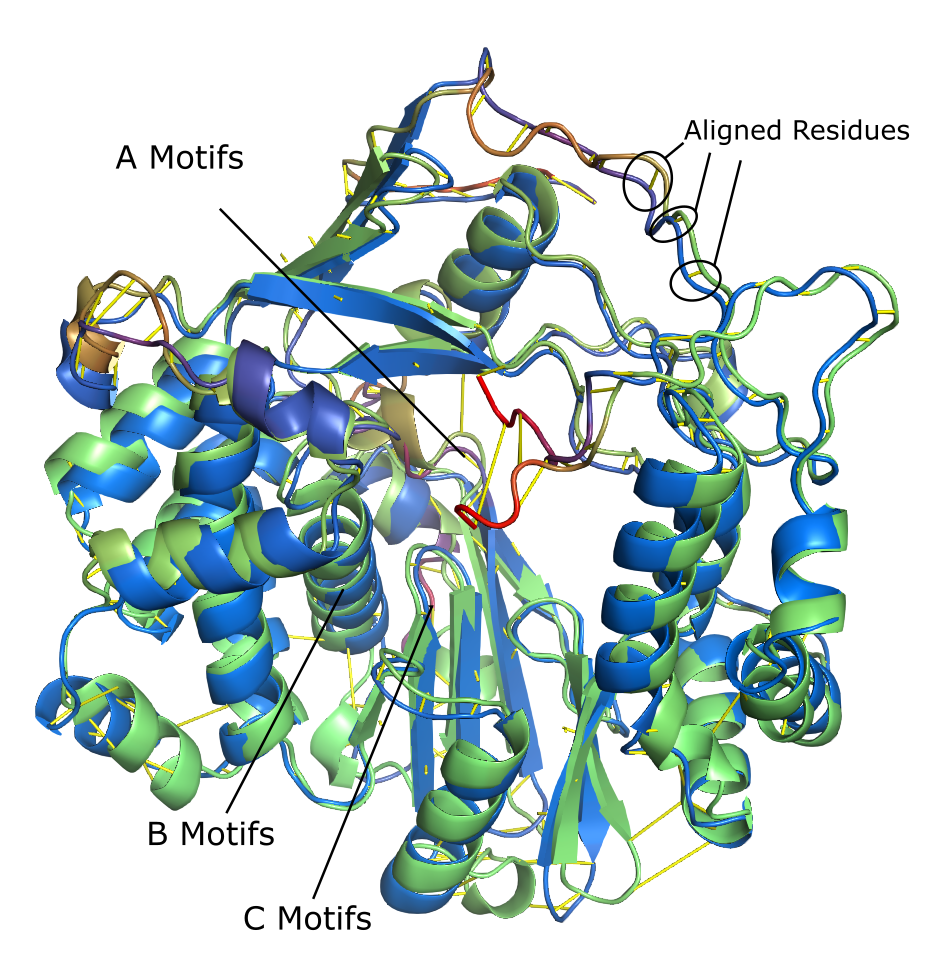
We can visualize the correspondence in PyMOL. The function pymol_protein_viewer.compare_proteins_in_pymol uses weighted_alignment.weighted_RMSD to superimpose the two proteins by minimizing weighted RMSD, and displays dashes between pairs of aligned residues.

import GWProt.pymol_protein_viewer

GWProt.pymol_protein_viewer.compare_proteins_in_pymol(
    file1 = dir + A.name_list[0] + '.pdb',
    file2 = dir + A.name_list[10] + '.pdb',
    chain1 ='A',
    chain2 ='A',
    correspondence=A.transport_dict[A.name_list[0]][A.name_list[10]],
    output_file= 'Example_Data/Pymol Outputs/Permutations.pse')

In this screenshot, the two proteins are overlaid: the ABC protein is green, the CAB protein is blue, and redder sections indicate higher local geometric distortion (LGD). The correspondence is shown by yellow lines connecting paired residues.

We can use switch_probabilities.get_switch_probabilities to identify switched residues, and switch_probabilities.visualize_switch_probabibilities for visualization.

import GWProt.switch_probabilities

GWProt.switch_probabilities.visualize_switch_probabibilities(GWProt.switch_probabilities.get_switch_probabilities(A.transport_dict[A.name_list[0]][A.name_list[10]], prot_num=0))

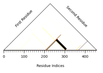
The white and light-colored areas represent residue pairs whose order is preserved, while dark rectangles indicate pairs whose order is switched. prot_num = 0 refers to the residues of the first protein (an ABC protein). The largest dark rectangle shows that residues 211–303 switch with residues 305–318, corresponding to the A–B and C regions, respectively.

Using switch_probabilities.preprocess and switch_probabilities.max_rectangle_diagonal, we can find the size of the largest such rectangle for each protein pair. This can help distinguish permutation types.

switch_score_mat = np.zeros((20,20))

for i in range(20):
    for j in range(20):
        if i ==j:
            continue

        T = A.transport_dict[A.name_list[i]][A.name_list[j]]

        SP0 = GWProt.switch_probabilities.get_switch_probabilities(T)
        SP1 = GWProt.switch_probabilities.preprocess(SP0)
        s = GWProt.switch_probabilities.max_rectangle_diagonal(SP1)[0]
        switch_score_mat[i,j] = s

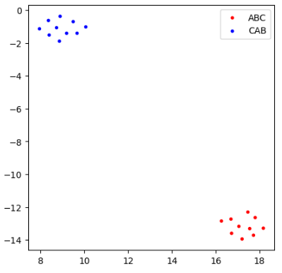
We can now cluster proteins based on the size of these rectangles, which provides better separation of permutation types.

reducer = UMAP(metric = 'precomputed')
embedding = reducer.fit_transform(switch_score_mat + switch_score_mat.T)
plt.figure(figsize=(5,5))
plt.scatter(embedding[:10,0] ,embedding[:10,1], color = ['red']*10 , s = 8 )
plt.scatter(embedding[10:,0] ,embedding[10:,1], color = ['blue']*10 , s = 8 )
plt.legend(["ABC","CAB" ])

The methods in switch_probabilities work well on this dataset because the proteins are morphologically similar in the GW metric. For proteins with greater variation, these techniques may be less effective.