Example 3: Clustering based on structural similarity

import numpy as np
import itertools as it
import multiprocess
import matplotlib.pyplot as plt
import time
import os
from umap.umap_ import UMAP

from GWProt.GW_protein import *
from GWProt.GW_protein_pI import *

/home/elijah/.local/lib/python3.10/site-packages/tqdm/auto.py:21: TqdmWarning: IProgress not found. Please update jupyter and ipywidgets. See https://ipywidgets.readthedocs.io/en/stable/user_install.html
  from .autonotebook import tqdm as notebook_tqdm

Riboviruses are a diverse group of viruses that include many human pathogens. They all encode an RNA-dependent RNA polymerase (RdRp), which is essential for replication, evolves rapidly, and often shows very low sequence homology. For these reasons, structural comparison is frequently more informative than sequence alone for identification and classification (see 1 and 2).

In this notebook we use a curated set of ~300 computationally folded RdRp core domains to illustrate how Gromov–Wasserstein (GW) distances can quantify structural similarity. We compare different GW variants available in GWProt (including fused-GW) to show their tradeoffs in clustering accuracy and runtime. The PDB files and metadata for this example are in the GWProt repository: https://github.com/CamaraLab/GWProt/tree/main/docs/Examples/Example_Data/RdRp%20Proteins.

Below we define a small helper for computing all-vs-all GW distance matrices in parallel.

import multiprocess
import itertools as it
import numpy as np
import time
import GWProt.GW_protein

def compute_in_parallel(proteins, comparison_method, **kwargs):
    N = len(proteins)
    dist_mat = np.zeros((N,N))
    start_time = time.time()

    with multiprocess.Pool() as pool:
        for r in  pool.imap(lambda pair: (pair[0], pair[1], comparison_method(proteins[pair[0]], proteins[pair[1]], **kwargs)), it.combinations(range(N),2), chunksize = 32):
            i,j,d = r
            dist_mat[i,j] = d
            dist_mat[j,i] = d

    run_time = int(time.time() - start_time)

    print(f'run time = {run_time//60} min, {run_time % 60} sec')
    return dist_mat

The main class in GWProt is GW_protein. An instance stores the data needed for structural comparisons: alpha-carbon coordinates, amino-acid sequence, and the intra-protein distance matrix (pairwise distances between alpha-carbons). You can initialize GW_protein objects from PDB files. In this example we assume the PDBs are in the folder palmstrub_little/ and load them into GW_protein instances:

import os

palmstrub_dir = "Example_Data/RdRp Proteins/palmstrub_little/"

all_files = os.listdir(palmstrub_dir)
base_prots = [GWProt.GW_protein.GW_protein.make_protein_from_pdb(palmstrub_dir + file) for file in all_files]

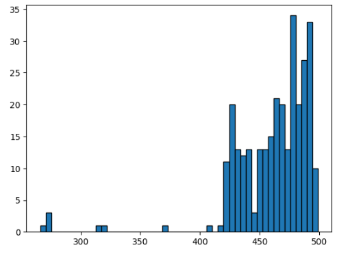
We can look at the distribution of the number of alpha-Carbons:

import matplotlib.pyplot as plt

plt.hist([len(m) for m in base_prots], bins=50, edgecolor='black')

Computing GW distances using all alpha-carbons is computationally intensive. For this dataset the following command may take several hours on a typical desktop (8 cores, 64 GB RAM). Consider downsampling or running on a cluster for faster results.

GW_dist_mat = compute_in_parallel(proteins=base_prots, comparison_method= GWProt.GW_protein.GW_protein.run_GW)

We can embed the GW pairwise distance matrix using UMAP and color points by ribovirus class to inspect separation between classes visually. The following code builds an interactive Plotly scatter plot for exploration.

import pandas as pd
import umap
import plotly.express as px
import pandas as pd
import plotly.io as pio

df = pd.read_csv('Example_Data/RdRp Proteins/TableS2.csv', index_col='GenPept accession')

reducer = umap.UMAP(metric='precomputed')
embedding = reducer.fit_transform(GW_dist_mat)

clas = [df['Class'].loc[m.name.split(".")[-1]] for m in base_prots]

df2 = pd.DataFrame({
    'UMAP1': embedding[:, 0],
    'UMAP2': embedding[:, 1],
    'Class' : clas
})

pio.renderers.default = 'notebook_connected'  # Set to the appropriate plotly renderer

fig = px.scatter(
    df2,
    x='UMAP1',
    y='UMAP2',
    color='Class',
    color_discrete_sequence=px.colors.qualitative.Set2  # You can change this palette
)

fig.update_layout(
    plot_bgcolor='white',
    paper_bgcolor='white',
    xaxis=dict(showgrid=False, zeroline=False, showticklabels=False, scaleanchor='y'),
    yaxis=dict(showgrid=False, zeroline=False, showticklabels=False)
)

fig.update_traces(marker=dict(size=3, opacity=0.8))
fig.show()

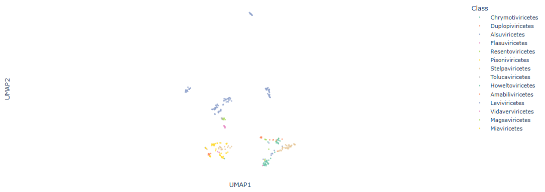
We train a nearest-neighbor classifier in the GW embedding to predict the ribovirus class and evaluate performance using Matthews Correlation Coefficient (MCC) with 5-fold cross-validation. MCC is a balanced metric that accounts for true/false positives and negatives. In this example the classifier yields an MCC of 0.912, indicating strong class separability in the GW-derived space.

from sklearn.neighbors import KNeighborsClassifier
from sklearn.model_selection import StratifiedKFold, cross_val_predict
from sklearn.metrics import matthews_corrcoef

clf = KNeighborsClassifier(metric="precomputed", n_neighbors=3, weights="distance")
cv = StratifiedKFold(n_splits=5, shuffle=True,random_state=0)
cvp = cross_val_predict(clf, X=GW_dist_mat, y=clas, cv=cv)

print(matthews_corrcoef(cvp, clas))

We can downsample each protein to an evenly spaced subset of residues to speed up GW computations. Downsampling reduces runtime significantly at the cost of some structural detail — higher downsampling is faster but typically reduces accuracy. Use this option when exploring large datasets or when GPU/cluster resources are limited.

downsampled_100_prots = [p.downsample_n(n=100) for p in base_prots]
GW_dist_mat = compute_in_parallel(proteins=downsampled_100_prots, comparison_method= GWProt.GW_protein.GW_protein.run_GW)

On this machine, the downsampled run completed in about 4 minutes, with MCC dropping slightly to 0.899.

Another strategy is to rescale the intra-protein distance matrices (e.g., applying a concave transform such as square root). Rescaling increases the relative weight of short-range distances and often improves classification accuracy with little runtime penalty. Below we apply rescaling together with downsampling; the order (downsampling → scaling vs. scaling → downsampling) typically does not affect the final result.

scaled_prots = [p.scale_ipdm(inplace = False) for p in downsampled_100_prots]
GW_dist_mat = compute_in_parallel(proteins=scaled_prots, comparison_method= GWProt.GW_protein.GW_protein.run_GW)

After rescaling the intra-protein distances we observe improved performance (MCC = 0.921 in this example), higher than the simple downsampled result.

Next, we demonstrate fused Gromov–Wasserstein (FGW) using a BLOSUM-derived difference matrix. FGW can incorporate sequence- or feature-based differences in addition to geometry; its effect on accuracy depends on the chosen feature distances. FGW generally has a runtime comparable to standard GW.

import GWProt.FGW_matrices

GW_dist_mat = compute_in_parallel(proteins=scaled_prots, comparison_method=GWProt.GW_protein.GW_protein.run_FGW_dict, alpha = 0.05,d = GWProt.FGW_matrices.get_BLOSUM_dict(n = 62))

GWProt provides several feature-based distance options for fused GW in addition to BLOSUM-based scores. Examples include residue isoelectric point distances (module GW_protein_pI) and hydrophobicity-based distances; users can also supply custom distance matrices. These fused metrics can improve performance when feature differences are informative.