Example 1: Identifying switch regions in KRAS

KRAS (Kirsten Rat Sarcoma) is a signaling protein involved in cell proliferation. In its inactive state, it is bound to guanosine diphosphate (GDP). In its active state, it is bound to guanosine triphosphate (GTP) and activates effector proteins that interact with two flexible switch regions. Certain mutant forms of KRAS remain constitutively active, which can cause uncontrolled proliferation and lead to various cancers. Thus, mutant KRAS is a key drug target.

In this example, we analyze 54 experimentally determined structures of KRAS using GWProt. We group them by Gromov-Wasserstein (GW) distance and examine how this relates to conformational changes in the switch regions. We also demonstrate how the local geometric distortion (LGD) highlights these flexible regions.

The dataset consists of PDB files for KRAS (wild type and several mutants) retrieved from the RCSB Protein Data Bank. Ligands, ions, and small molecules have been removed for clarity. All proteins are truncated to amino acids 2–162 in the canonical sequence to ensure consistency. Files with multiple chains were split into separate entries.

The processed PDB files are available in the following folder in the GitHub repository. For this notebook, we use the local copy:

dir = "Example_Data/KRAS Proteins/"

We start by creating GW_protein objects for each protein structure:

import GWProt.GW_protein
import os

protein_list = [GWProt.GW_protein.GW_protein.make_protein_from_pdb(pdb_file = os.path.join(dir, file))  for file in os.listdir(dir)]

We now initialize an LGD_Comparison object to compare these protein structures using the Gromov-Wasserstein (GW) distance and local geometric distortion (LGD). In this example, we store the correspondences in memory with RAM = True. This will use approximately 600 MB of memory; note that memory usage grows quadratically with the number of proteins.

import GWProt.lgd_comparison

A = GWProt.lgd_comparison.LGD_Comparison(prot_list = protein_list, RAM =  True)

We now compute all pairwise GW distances. On a machine with 16 parallel processes, this takes about 5 seconds; with a single process, it takes around 40 seconds.

# Run GW all-vs-all. Adjust 'processes' for your hardware.
A.GW_compute_lgd(processes = 16)

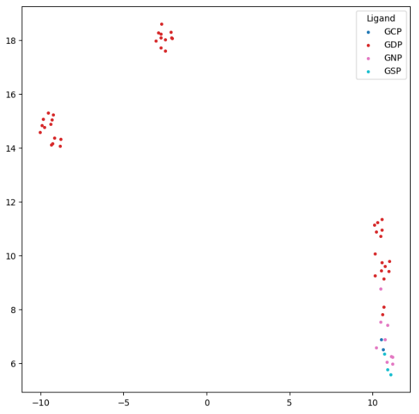
We next examine how the conformation of KRAS varies with the bound ligand. The original PDB files include KRAS bound to GDP and to GTP analogues (GNP, GCP, and GSP). This information is stored in a metadata file, which we now load.

import csv

ligand_dict = {}
with open("Examples/Example_Data/KRAS Ligands.csv", 'r') as ligand_metadata:
    csvreader = csv.reader(ligand_metadata)
    for row in csvreader:
        ligand_dict[row[0]] = row[1]

ligand_list  = [ligand_dict[p.name] for p in protein_list]

To visualize the structural relationships, we create a UMAP plot from the GW distance matrix:

import matplotlib.pyplot as plt
import numpy as np
from umap import UMAP

distance_matrix = A.get_GW_dmat()
reducer = UMAP(metric = 'precomputed', random_state=1)
embedding = reducer.fit_transform(distance_matrix)

plt.figure(figsize=(8, 8))
unique_ligands = np.unique(ligand_list)
colors = plt.cm.tab10(np.linspace(0, 1, len(unique_ligands)))

for ligand, color in zip(unique_ligands, colors):
    mask = np.array(ligand_list) == ligand
    plt.scatter(
        embedding[mask, 0],
        embedding[mask, 1],
        c=[color],
        s=7,
        label=ligand
    )

plt.legend(title="Ligand")
plt.show()

We can also cluster the proteins in this structural space:

from sklearn.cluster import KMeans

kmeans = KMeans(n_clusters=4, n_init=10, random_state=1)
cluster_labels = kmeans.fit_predict(embedding)

plt.figure(figsize=(8, 8))
cmap = plt.cm.tab10

for cluster_id in range(4):
    mask = cluster_labels == cluster_id
    plt.scatter(
        embedding[mask, 0],
        embedding[mask, 1],
        s=10,
        c=[cmap(cluster_id)],   # one color per cluster
        label=f"Cluster {cluster_id}"
    )

plt.legend(title="Cluster")
plt.show()

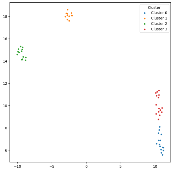
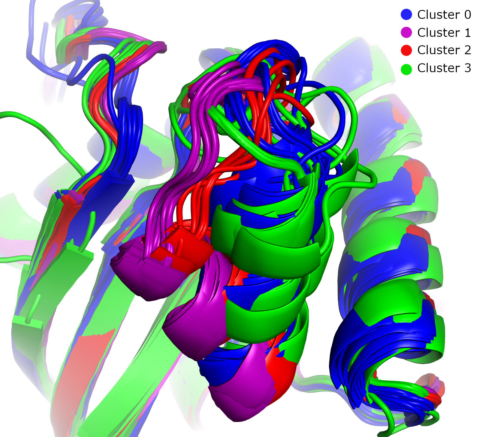
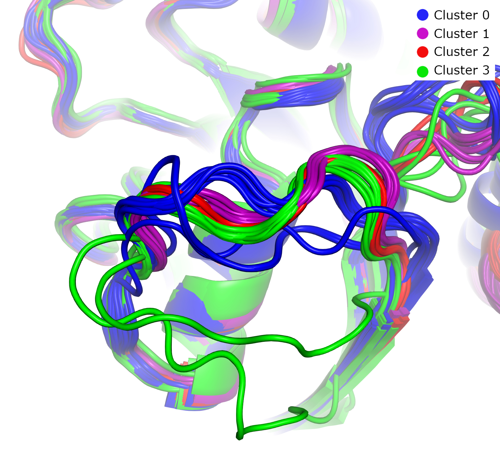
Using PyMOL, we can clearly see that these clusters correspond to distinct conformational states. In this image of switch region II, the four clusters exhibit different conformations. Clusters 0 and 3 are close both conformationally and in the UMAP embedding, reflecting their low GW distances.

In this image of switch region I, most GTP-analogue-bound proteins (blue) have similar conformations, while most GDP-bound proteins (red, green, and purple) form a distinct group.

Next, we use pymol_protein_viewer.show_proteins_with_values to visualize the proteins and the local geometric distortion (LGD) values for each residue. A.raw_lgd_dict contains the LGD values from all pairwise calculations; we first average these for each protein, then generate a PyMOL file for visualization.

import GWProt.pymol_protein_viewer

avg_lgd_dict =  GWProt.lgd_comparison.normalize_lgd_dict(A.raw_lgd_dict)
avg_lgd_list = [avg_lgd_dict[name] for name in A.name_list]

GWProt.pymol_protein_viewer.show_proteins_with_values(
    infiles = [os.path.join(dir, file) for file in os.listdir(dir)],
    chain_ids = [file[5] for file in os.listdir(dir)],
    data_lists = avg_lgd_list,
    output_file = "Examples Data/Pymol Outputs/KRAS_LGD.pse")

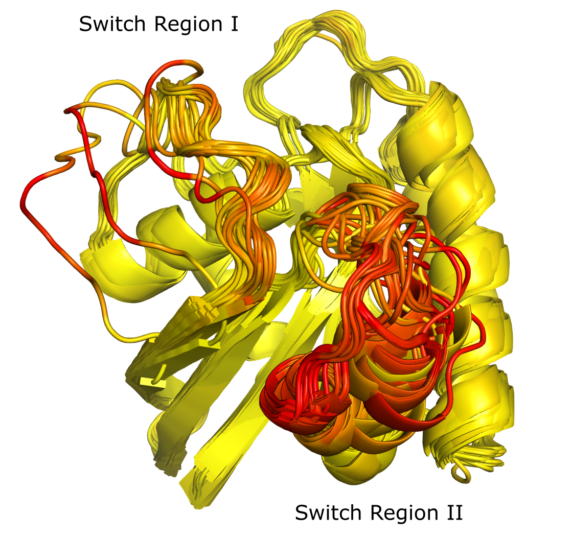
The PyMOL file generated and saved as KRAS_LGD.pse can be opened in PyMOL. The switch I region is in the upper left foreground, and switch II is in the right foreground. Both regions show higher local geometric distortion (redder colors), while non-switch regions have lower LGD (yellow colors).

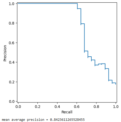
Next, we test how well the local geometric distortion (LGD) values can be used to predict the switch I and switch II regions. These regions do not have precisely defined endpoints, but for this analysis we use residues 30–40 and 60–72 in the canonical sequence. In these files, these correspond to indices 28–38 and 58–74.

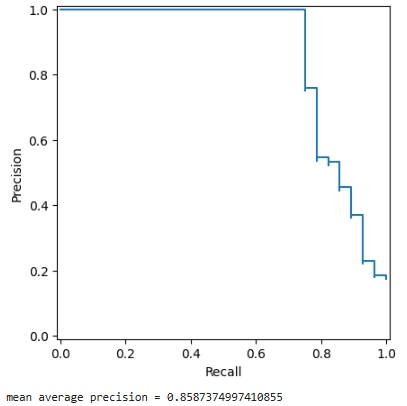
We display the precision-recall curve for a randomly selected protein and report the mean average precision (area under the precision-recall curve).

import sklearn.metrics

switch_regions_dict = {p.name : [int(i in range(28,39) or i in range(58,75)) for i in range(161)] for p in protein_list}

p, r, _ = sklearn.metrics.precision_recall_curve(switch_regions_dict['5mla_A'], avg_lgd_dict['5mla_A'])
sklearn.metrics.PrecisionRecallDisplay(precision=p, recall=r).plot()
plt.show()
avg_precision_dict = GWProt.lgd_comparison.get_AP_scores(avg_lgd_dict, switch_regions_dict, upper=True)

print(f'mean average precision = {np.mean(list(avg_precision_dict.values()))}')

We can also compute transferred local geometric distortion values using raw_transferred_lgd, which we then average with normalize_lgd_dict. Transferring uses the calculated correspondences to map LGD values from one protein to another in an all-to-all fashion. This generally improves accuracy.

transferred_lgd = GWProt.lgd_comparison.normalize_lgd_dict(A.raw_transferred_lgd(avg_lgd_dict))

p, r, _ = sklearn.metrics.precision_recall_curve(switch_regions_dict['5mla_A'], transferred_lgd['5mla_A'])
sklearn.metrics.PrecisionRecallDisplay(precision=p, recall=r).plot()
plt.show()

transferred_avg_precision_dict = GWProt.lgd_comparison.get_AP_scores(transferred_lgd, switch_regions_dict, upper=True)
print(f'mean average precision = {np.mean(list(transferred_avg_precision_dict.values()))}')